Note: The first version of this file was written in Mathematica 4.2. However, the author hopes that all algorithms and functions were successfully (and regurarly) rewritten to be in line with up-to-date version of Mathematica.
Option pricing via Monte Carlo simulation (Odhad ceny opce dle simulace Monte Carlo)
Symbols and Notations
Bellow, we review the notations and symbols which are most frequently used in this text.
| spot | spot price of the underlying asset at time zero | spotová cena podkladového aktiva v čase nula | |
| spotT | spot price of the underlying asset at maturity time | spotová cena podkladového aktiva v době zralosti | |
| K | exe | exercise price (strike price) | realizační cena |
| T | mat | maturity time | doba zralosti |
| τ | timeto | time to maturity | doba do zralosti |
| r | r | riskless rate | bezrizikový výnos |
| σ | vol | volatility of returns of S | volatilita výnosů S |
| q | q | dividend yield | dividendový výnos |
| N | number | number of independent scenarios | počet nezávislých scénářů |
| □ | length | length of the time interval used for simulation | délka časového úseku pro simulaci |
| θ | driftVG(NIG) | skewness parameter | parametr řídící šikmost |
| ν | gammavariance | kurtosis parameter | parametr řídící špičatost |
| ω | omega | mean correcting parameter | parametr upravující střední hodnotu |
| dist[θ] | distribution | a general notation to a target distribution with parameters θ | obecné označení cílového rozdělení pravděpodobnosti s parametry θ |
| G[a,b] | gamma dist. | gamma distribution with shape and scale parameters a and b | gama pravděpodobnostní rozdělení s parametry a a b |
Required functions of Mathematica: Table, Mean, StandardDeviation, Variance, Skewness, Kurtosis, Module, SeedRandom, RandomReal, Clear, Take, Drop, Append, Delete, Flatten, Timing, Join, Quantile, CharacteristicFunction, PDF, UniformDistribution, Grid, GraphicsArray, Histogram, Plot, NormalDistribution, CDF, GammaDistribution, ...
![]()
![]()
Some basic facts about probability, random numbers and statistical estimation
This section is under construction...
Random numbers from prespecified distributions
In this section we provide basic moduls to generate random numbers from selected distributions, useful in Financial modeling. However, we start with general moduls, without specifying the target distribution.
Define first the vector of parameters for further utilization (head of resulting tables, head), the function for grid to provide the table of particular results, ResultsGrid, and the parameter to set the maximal number of trials (kk):

General modules
PMC (Plain Monte Carlo)
This is the simplest approach, since we use solely the predefined algorithm of Mathematica specified within the function RandomReal[dist[θ],{number}]. Here, dist[θ] refers to the target distribution with a given set of parameters θ, number is the number of independent scenarios we generate. Within the algorithm bellow, when we specify the internal module for pN, we use nn to allow us to recover exactly the same "random" realizations later, if needed. Thus, the algorithm PMCrannumPar has three variables, dist[θ], nn, and number. It produces the vector of random variables, rannum, for which the estimations of the sample mean, standard deviation, variance, skewness, and kurtosis is obtained. Moreover, the algorithm returns also the number of generated scenarios. Finally, we show how to run the algoritm to get the vector of estimated parameters accompanied by the overall time costs for ![]() random scenarios. Note: We start the definition by clearing the function (PMCrannumPar)
random scenarios. Note: We start the definition by clearing the function (PMCrannumPar)
In[39]:=

![]()
Alternatively, we can define a simple algorithm that will not produce the estimation of the paramaters, but solely the random numbers. Although it takes more memory to rember the results, it is the only way how to picture (approximate) the probability density function. Basically, we have three choices - the approximation of the PDF by a histogram; smoothing it by a Kernel function; comparing the quantiles (QQ plot). As above, we first realize ![]() random scenarios.
random scenarios.
In[42]:=
![]()
![]()
Another way we can proceed is to produce everything within a single algoritm. Subsequently, we pick up separately the parameters of a given random number distribution, including the time costs, and the set of random numbers, see bellow.

![]()
To conclude, when we are interested mainly in desriptive statistic parameters, we use the modul with "Par", PMCrannumPar. By contrast, when we need to get the numbers for further utilization, we can use the modul with "Num", PMCrannumNum. Finally, to get both, we use just PMCrannum.
The approach described above can be used in connection with any predefiened distribution. Obviously, if there is a need for a distribution which is not predefined in Mathematica (eg. VarianceGamma), it must be defined before running the procedure.
AVMC (Monte Carlo with antithetic variates)
The Monte Carlo approach with antithetic variates in its basic form gives an additional path for each original one obtained due to the predefined algorithm of Mathematica, see PMC. Thus, we call only for a given fraction of the required amount of variables, rannum. More particularly, in its simplest form we obtain directly one half of the variables we actually need, rannumpart=number/2 The drawback of the approach is that it can be used directly only for symmetric distributions. If the mean is nonzero, we have to deduce the random realizations from its value MEAN.

![]()
Similarly to PMC, we can define two alternative algoritms. First, we state the one to produce the set of random numbers:
![]()
![]()
And here is the other one:

![]()
If the target distribution is not symmetric, we can reformulate the algorithm to produce first random numbers due to the standard uniform distribution, ie we obtain randomly the probabilities, and then apply the inverse transform method.
ITMC (Inverse Transforme Monte Carlo)
Assume that we are able to generate random variables from the standard uniform distribution, but we are interested in some more complex one. In other words, the standard uniform variates provide us randomly with probabilities, ie values of the target distribution function. Assuming that the inverse function to the target distribution function exists, we can transform such variables to obtain the target ones. In Mathematica, we can use the function called Quantile. We state only the basic algorithm.

![]()
A strong drawback of ITMC is that the calculation of inverse functions often takes too much time - it is several times more time consuming than PMC.
SSMC (Stratified Sampling Monte Carlo)
The key step of this improvement to simple Monte Carlo approach is to stratify the interval of admissible resutls into subintervals with equal probabilities of occurence (alternativelly, we call these subintervals stratas). In general, there exist two approaches to stratified sampling. We can stratify either the original set or the unit interval, ie probabilites. The latter case is generally more tractable, since it is not required to deal with infinite bounds and the subintervals have equal length. We first define an internal module to provide random numbers due to the standard uniform distribution, pU. Next, we table whole numbers (vector P1) up to the total quantity of scenarios considered, number. Subsequently, we stratify the unit interval and generate one random number for each of them. Finally, we produce random numbers from the target distribution applying function Quantile.

![]()
As we will seevlater this algorithm extends ITMC approach to provide more efficient results at almost same time costs. Clearly, the algorithm can be redefined to produce more independent random numbers for each of the stratas. As above, we state the two alternative algorithms bellow. This is the first one:

![]()
And here is the other one:

![]()
It is obvious, that such approach works only for one-dimensional problems. If more dimensional random vector must be considered, this approach can be easily extended to LHS (Latin Hypercube Sampling) Monte Carlo method. The application is easy. We only need to permute randomly the vector of boundaries for particular stratas P.
AV-SSMC (Stratified Sampling with Antithetic Variates Monte Carlo)
The stratified Monte Carlo approach presented above is based on generating random numbers from Uniform Distribution first. Clearly, we can also think about improving the generator by e.g. AVMC approach. In this subsection we present several alternatives. For simplicity, we will deal only with algorithms of SSMCrannumNum class. We start with algorithm, that provides two paths for each strata: we accompine the original one by a mirrored one, due to the mean of the strata.

Alternatively, both realizations can be symmetric with respect to the mean of the entire interval.

Next choice can be to...
Uniform Distribution
Definition
Uniform distribution indicates that all admissible values can arise with the same probability, ie the probabilities of particular outcomes are equal. In Mathematica, we can get uniformly distributed random numbers calling UniformDistribution[{a, b}], where a and b indicates the bounds of admissible values, b>a. It can be defined either by a characteristic function:
![]()
![]()
or a distribution function:
![]()
![]()
Clearly, it is a horizontal line for any x∈[a,b].
Generally we apply a standard uniform distribution, ie uniform distribution with unit margins, a=0 and b=1, which we can call for by typing UniformDistribution[{0,1}] or in order to get random variables RandomReal[{}]. Now, we ask Mathematica to calculate analytically the first four moments of the distribution function and we accompany them by the number of scenarios and the time costs.
![]()
![]()
Algorithms
This part is under construction...
PMC (Plain Monte Carlo)
Now, we utilize the algorithm PMCrannumPar defined above. Before getting the table of results, we must specify kk, the first row head and the last row lr with analytically obtained parameters.
![]()
![]()
| Scenarios | Mean | StandardDeviation | Variance | Skewness | Kurtosis | Time |
| 10 | 0.408312 | 0.284703 | 0.0810556 | 0.324249 | 1.54837 | 1.48326*10^^-13 |
| 100 | 0.464006 | 0.267273 | 0.0714351 | 0.112971 | 1.94004 | 1.48326*10^^-13 |
| 1000 | 0.501675 | 0.285255 | 0.0813701 | -0.0580989 | 1.8471 | 1.48326*10^^-13 |
| 10000 | 0.50299 | 0.287051 | 0.0823985 | -0.0163006 | 1.82057 | 1.48326*10^^-13 |
| 100000 | 0.498979 | 0.288403 | 0.0831763 | 0.00472851 | 1.80442 | 0.031 |
| 1000000 | 0.499671 | 0.288485 | 0.0832236 | -0.000298105 | 1.80108 | 0.219 |
| Analytically | 0. | 0.144553 | 0.0208957 | -0.80556 | 4.14235 |
In order to compare the density/distribution we apply the other algorithm.
![]()
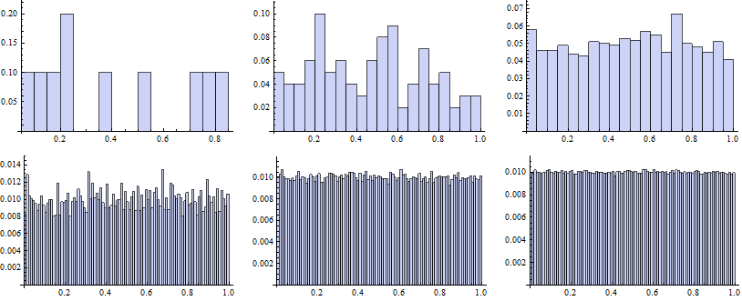
Now we map the Histogram function to vectors of random numbers generated for particular k.
![]()
AVMC (Monte Carlo with antithetic variates)
AVMC approach needs to run only one half of scenarios comparing with PMC. We examine if a decrease in time costs is adequate. We should be also interested, if the estimated parameters converge to the true values rapidly.
![]()
![]()
| Scenarios | Mean | StandardDeviation | Variance | Skewness | Kurtosis | Time |
| 10 | 0.5 | 0.333306 | 0.111093 | 0. | 1.07933 | 1.50704*10^^-17 |
| 100 | 0.5 | 0.264249 | 0.0698278 | -8.38837*10^^-21 | 1.91573 | 1.50704*10^^-17 |
| 1000 | 0.5 | 0.291552 | 0.0850024 | -3.28607*10^^-21 | 1.744 | 1.50704*10^^-17 |
| 10000 | 0.5 | 0.28749 | 0.0826508 | -3.08041*10^^-21 | 1.81256 | 1.50704*10^^-17 |
| 100000 | 0.5 | 0.287799 | 0.082828 | 1.28653*10^^-20 | 1.80739 | 0.031 |
| 1000000 | 0.5 | 0.288598 | 0.0832889 | -1.82542*10^^-20 | 1.80062 | 0.265 |
| Analytically | 0.5 | 0.288675 | 0.0833333 | 0. | 1.8 |
Alternatively, we use the other algorithm to compare the overall distribution.
![]()
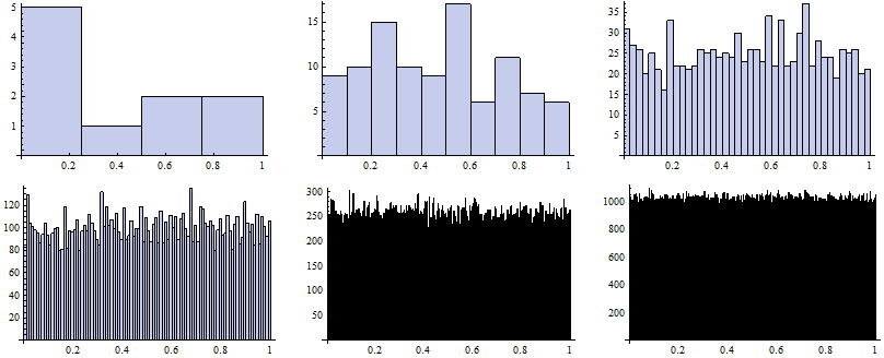
Now we map the Histogram function to vectors of random numbers generated for particular k.
![]()
![]()
ITMC (Monte Carlo on the basis of inverse transform method)
In order to separate the effect of stratification and the inverse function to the distribution function evaluation, we should run ITMC alone.
![]()
![]()
| Scenarios | Mean | StandardDeviation | Variance | Skewness | Kurtosis | Time |
| 10 | 0.408312 | 0.284703 | 0.0810556 | 0.324249 | 1.54837 | 7.37257*10^^-17 |
| 100 | 0.464006 | 0.267273 | 0.0714351 | 0.112971 | 1.94004 | 7.37257*10^^-17 |
| 1000 | 0.501675 | 0.285255 | 0.0813701 | -0.0580989 | 1.8471 | 7.37257*10^^-17 |
| 10000 | 0.50299 | 0.287051 | 0.0823985 | -0.0163006 | 1.82057 | 0.016 |
| 100000 | 0.498979 | 0.288403 | 0.0831763 | 0.00472851 | 1.80442 | 0.062 |
| 1000000 | 0.499671 | 0.288485 | 0.0832236 | -0.000298105 | 1.80108 | 0.609 |
| Analytically | 0.5 | 0.288675 | 0.0833333 | 0. | 1.8 |
![]()
SSMC (Stratified Monte Carlo)
Now we can proceed to stratified Monte Carlo. Since it generally shows to be very time consuming to evaluate the inverse function to any distribution function, we switch to the following algorithm:
![]()
![]()
| Scenarios | Mean | StandardDeviation | Variance | Skewness | Kurtosis | Time |
| 10 | 0.490831 | 0.302334 | 0.0914058 | 0.132533 | 1.81545 | 0. |
| 100 | 0.49964 | 0.289999 | 0.0840992 | -0.00361333 | 1.79589 | 0. |
| 1000 | 0.500002 | 0.288832 | 0.083424 | -6.86584*10^^-6 | 1.80008 | 0. |
| 10000 | 0.5 | 0.288689 | 0.0833415 | -2.36153*10^^-6 | 1.8 | 0.015 |
| 100000 | 0.5 | 0.288677 | 0.0833342 | 2.21808*10^^-7 | 1.8 | 0.047 |
| 1000000 | 0.5 | 0.288675 | 0.0833334 | -1.48766*10^^-9 | 1.8 | 0.748 |
| Analytically | 0.5 | 0.288675 | 0.0833333 | 0. | 1.8 |
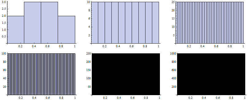
Now we map the Histogram function to particular vectors of random numbers generated for particular k.
![]()
![]()
Normal (Gaussian) Distribution
Definition
The term normal distribution is commonly used instead of Gaussian distribution, since such a distribution of random variables is supposed to be the most frequent in practice considerations. In Mathematica, we call for it by typing NormalDistribution[μ, σ], ie with mean μ and its standard deviation σ>0. It can be defined either by a characteristic function:
![]()
![]()
or a distribution function:
![]()

We plot the probability distribution functions for various σ and μ, respectivelly, bellow.
![]()

Note: with plain settings the first function is drawn with blue, the second with violet, etc.
Generally we apply a standard normal distribution, ie normal distribution with zero mean and unit variance, for which we can call simply by NormalDistribution[ , ]. The reason is that it can be easilly transformed, with insignificant time costs, into the target distribution by multiplying the original vector by σ and adding μ. Now, we analytically calculate the first four moments of the distribution function and we accompany them by the number of scenarios and the time costs.
![]()
![]()
Algorithms
This part is under construction...
PMC (Plain Monte Carlo)
Here, we utilize the algorithm PMCrannumPar defined above. Before getting the table of results, we must specify kk, the first row head and the last row lr with analytically obtained parameters.
![]()
![]()
| Scenarios | Mean | StandardDeviation | Variance | Skewness | Kurtosis | Time |
| 10 | 0.353029 | 0.78523 | 0.616586 | -0.673941 | 3.27474 | 0. |
| 100 | -0.00966945 | 1.01417 | 1.02854 | 0.136525 | 2.85647 | 0. |
| 1000 | -0.0457642 | 0.972646 | 0.94604 | 0.016272 | 2.89682 | 0. |
| 10000 | -0.0042003 | 0.98622 | 0.972629 | 0.0255267 | 2.9847 | 0. |
| 100000 | 0.00458268 | 0.999197 | 0.998395 | 0.0130988 | 2.99755 | 0.046 |
| 1000000 | -0.000799485 | 1.00061 | 1.00123 | 0.00340776 | 2.99843 | 0.344 |
| Analytically | 0 | 1 | 1 | 0 | 3 |
Next, in order to compare the density/distribution we apply the other algorithm.
![]()
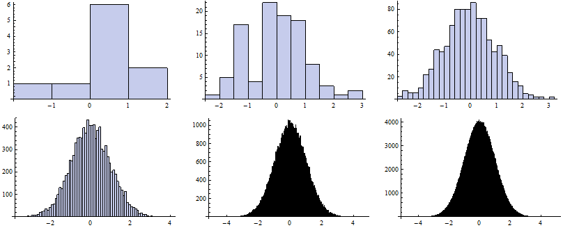
Now we map the Histogram function to vectors of random numbers generated for particular k.
![]()
![]()
To draw the QQ plot we first specify self-defined function to evaluate the CDF for each random number from the data set, specifing the DataRange on the x-axes. Next, we sort the original series of data and map the QQplot function to them.
![]()
![]()
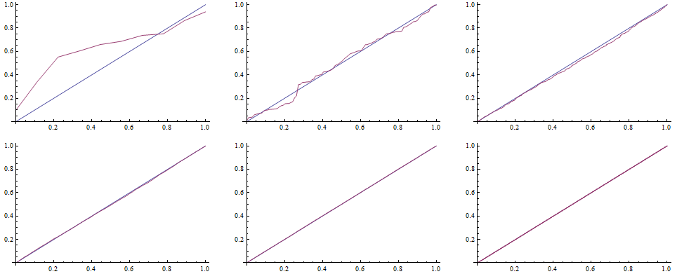
In order to complete the comparison, we can evaluate the Kolmogorov-Smirnov test, ie we look for the widest distance between the simulated distribution function and the teoretical one.
![]()
![]()
AVMC (Monte Carlo with antithetic variates)
AVMC approach needs to run one half of scenarios comparing with PMC. We examine if a decrease in time costs is adequate. We should be also interested, if the estimated parameters converge to true values rapidly.
![]()
![]()
| Scenarios | Mean | StandardDeviation | Variance | Skewness | Kurtosis | Time |
| 10 | 0. | 0.851245 | 0.724618 | 0. | 2.79288 | 0. |
| 100 | 0. | 0.984274 | 0.968796 | 1.84684*10^^-20 | 3.12288 | 0. |
| 1000 | 1.30104*10^^-21 | 0.978274 | 0.95702 | -3.9433*10^^-21 | 2.86486 | 0. |
| 10000 | 1.04083*10^^-21 | 0.975888 | 0.952358 | 7.93385*10^^-21 | 2.92746 | 0.015 |
| 100000 | -7.11237*10^^-22 | 0.996044 | 0.992104 | -3.61194*10^^-21 | 2.97502 | 0.031 |
| 1000000 | 1.44329*10^^-21 | 0.999972 | 0.999945 | -3.55786*10^^-20 | 3.00156 | 0.281 |
| Analytically | 0 | 1 | 1 | 0 | 3 |
Alternatively, we use the other algorithm to compare the overall distribution.
![]()
Now we map the Histogram function to vectors of random numbers generated for particular k.
![]()
![]()

To draw the QQ plot we first specify self-defined function to evaluate the CDF for each random number from the data set, specifing the DataRange on the x-axes. Next, we sort the original series of data and map the QQplot function to them.
![]()
![]()
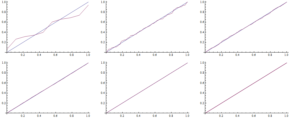
In order to complete the comparison, we can evaluate the Kolmogorov-Smirnov test, ie we look for the widest distance between the simulated distribution function and the teoretical one.
![]()
![]()
ITMC (Monte Carlo on the basis of inverse transform method)
In order to separate the effect of stratification and applying the inverse function to the distribution function within SSMC approach, we need to run ITMC alone.
![]()
![]()
| Scenarios | Mean | StandardDeviation | Variance | Skewness | Kurtosis | Time |
| 10 | -0.297192 | 0.851177 | 0.724503 | 0.149367 | 1.67205 | 6.46705*10^^-15 |
| 100 | -0.123177 | 0.88752 | 0.787692 | -0.039672 | 2.97797 | 0.031 |
| 1000 | -0.00439253 | 0.996385 | 0.992783 | -0.064306 | 3.30474 | 0.187 |
| 10000 | 0.0092563 | 0.993181 | 0.986409 | -0.00842903 | 2.98872 | 1.982 |
| 100000 | -0.00350102 | 1.00007 | 1.00013 | 0.000704593 | 3.02202 | 19.562 |
| 1000000 | -0.00136684 | 0.998922 | 0.997845 | -0.000932943 | 3.00355 | 197.357 |
| Analytically | 0 | 1 | 1 | 0 | 3 |
![]()
SSMC (Stratified Monte Carlo)
We can proceed now to stratified Monte Carlo. Since it generally seems to be very time consuming to evaluate the inverse function to any distribution function, we switch to the following algorithm:
![]()
![]()
| Scenarios | Mean | StandardDeviation | Variance | Skewness | Kurtosis | Time |
| 10 | 0.00173221 | 1.00372 | 1.00746 | 0.350424 | 2.40684 | 1.78746*10^^-14 |
| 100 | -0.00403324 | 0.990024 | 0.980148 | -0.0323878 | 2.71479 | 0.016 |
| 1000 | -0.000071616 | 0.999577 | 0.999154 | -0.00196509 | 2.95589 | 0.203 |
| 10000 | -2.1631*10^^-6 | 0.999975 | 0.99995 | 0.0000151301 | 2.99534 | 2.012 |
| 100000 | 7.80981*10^^-8 | 0.999998 | 0.999996 | 2.2293*10^^-6 | 2.99938 | 19.781 |
| 1000000 | 2.26954*10^^-8 | 1. | 1. | 1.99489*10^^-6 | 2.99994 | 197.591 |
| Analytically | 0 | 1 | 1 | 0 | 3 |
Now we map the Histogram function to particular vectors of random numbers generated for particular k.
![]()
![]()
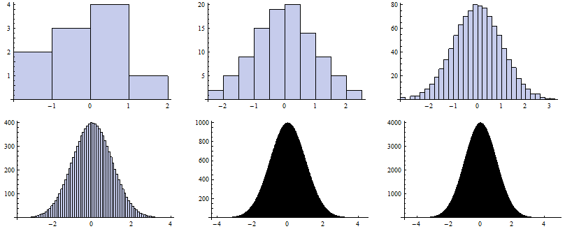
To draw the QQ plot we first specify self-defined function to evaluate the CDF for each random number from the data set, specifing the DataRange on the x-axes. Next, we sort the original series of data and map the QQplot function to them.
![]()
![]()
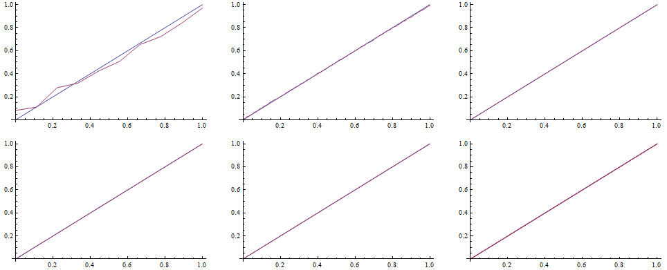
In order to complete the comparison, we can evaluate the Kolmogorov-Smirnov test, ie we look for the widest distance between the simulated distribution function and the teoretical one.
![]()
![]()
Gamma Distribution
Definition
Gamma distribution belongs to the large family of distributions with non-negative realizations. It is therefore useful when modeling of stochastic processes with non-negative realizations (eg. time increments) is considered. In Mathematica, we call for it by GammaDistribution[a, b], ie with parameters of shape a > 0 and scale b > 0. With basic conditions, we can defined it either by a characteristic function:
![]()
![]()
or a distribution function:
![]()
![]()
The mean and the variance can be precalculated as follows:
![]()
![]()
![]()
![]()
Due to
![]()
![]()
it follows that ![]() and
and ![]() Later, whitin modeling the asset price evolutions, we will require: μ=1 and ν=0.2264. Note also that the Gamma distribution is often defined by parameters α and β with relations to a and b. Under suitable choice of parameters, the Gamma distribution gives us either an Exponential distribution or a Chi-2 distribution.
Later, whitin modeling the asset price evolutions, we will require: μ=1 and ν=0.2264. Note also that the Gamma distribution is often defined by parameters α and β with relations to a and b. Under suitable choice of parameters, the Gamma distribution gives us either an Exponential distribution or a Chi-2 distribution.
We plot the probability distribution function bellow.
![]()

Note: with plain settings the first function is drawn with blue, the second with violet.
It is important to know that it is sufficient to generate GammaDistribution[a, 1]. The reason is that it can be easilly transformed into target distribution GammaDistribution[a, b] when the results are multiplied by b. Now we analytically calculate the first four moments of the distribution function and we accompany them by the number of scenarios and the time costs, respectivelly.

![]()
Algorithms
This part is under construction...
PMC (Plain Monte Carlo)
Here, we utilize the algorithm PMCrannumPar defined above setting the distribution to be GammaDistribution[a,b]. Moreover, before getting the table of results, we must specify kk, the first row head and the last row lr with analytically obtained parameters.
![]()
![]()
![]()
| Scenarios | Mean | StandardDeviation | Variance | Skewness | Kurtosis | Time |
| 10 | 0.982436 | 0.526539 | 0.277244 | 0.616026 | 2.24096 | 0. |
| 100 | 0.95087 | 0.409521 | 0.167708 | 0.579633 | 2.88648 | 0. |
| 1000 | 0.991652 | 0.463546 | 0.214875 | 0.886468 | 4.12201 | 0. |
| 10000 | 1.00034 | 0.471482 | 0.222295 | 0.979527 | 4.50121 | 0.016 |
| 100000 | 1.00128 | 0.477557 | 0.228061 | 0.965656 | 4.4205 | 0.062 |
| 1000000 | 1.00023 | 0.475257 | 0.22587 | 0.951665 | 4.36562 | 0.593 |
| Analytically | 1. | 0.475815 | 0.2264 | 0.95163 | 4.3584 |
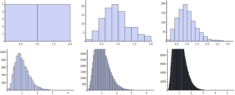
Now we map the Histogram function to vectors of random numbers generated for particular k.
![]()
![]()
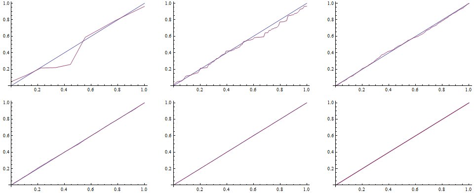
To draw the QQ plot we first specify self-defined function to evaluate the CDF for each random number from the data set, specifing the DataRange on the x-axes. Next, we sort the original series of data and map the QQplot function to them.
![]()
![]()
In order to complete the comparison, we can evaluate the Kolmogorov-Smirnov test, ie we look for the widest distance between the simulated distribution function and the teoretical one.
![]()
![]()
AVMC (Monte Carlo with antithetic variates)
Since the Gamma probability distribution is not a symmetric one, there is obviously no reason to apply the AVMC method in its basic form.
SSMC (Stratified Monte Carlo)
We can proceed now to stratified Monte Carlo. Since it generally seems to be very time consuming to evaluate the inverse function to any distribution function, we switch directly to the following algorithm to produce both (i) random numbers and (ii) inputs for the tables:
![]()
![]()
![]()
| Scenarios | Mean | StandardDeviation | Variance | Skewness | Kurtosis | Time |
| 10 | 0.994972 | 0.495258 | 0.24528 | 0.926469 | 3.17805 | 0.031 |
| 100 | 0.995893 | 0.465135 | 0.216351 | 0.761664 | 3.36312 | 0.203 |
| 1000 | 0.999832 | 0.475037 | 0.22566 | 0.922427 | 4.12768 | 1.888 |
| 10000 | 0.999989 | 0.475762 | 0.22635 | 0.948922 | 4.33162 | 19.359 |
| 100000 | 0.999999 | 0.475809 | 0.226394 | 0.951198 | 4.35303 | 203.597 |
| 1000000 | 1. | 0.475815 | 0.2264 | 0.951591 | 4.35782 | 1922.14 |
| Analytically | 1. | 0.475815 | 0.2264 | 0.95163 | 4.3584 |
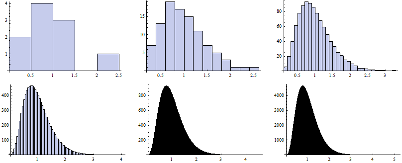
Now we map the Histogram function to vectors of random numbers generated for particular k.
![]()
![]()
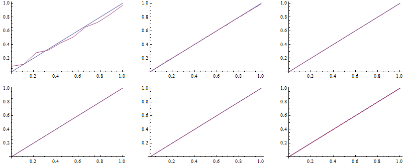
To draw the QQ plot we first specify self-defined function to evaluate the CDF for each random number from the data set, specifing the DataRange on the x-axes. Next, we sort the original series of data and map the QQplot function to them.
![]()
![]()
In order to complete the comparison, we can evaluate the Kolmogorov-Smirnov test, ie we look for the widest distance between the simulated distribution function and the teoretical one.
![]()
![]()
Variance Gamma Distribution
Definition
Variance gamma distribution is related to one of the most popular examples of Lévy processes, the Variance gamma process. There are several ways to its formulation, either as a difference of two gamma processes, which are, clearly, independent, or as a (geometric) Brownian motion subordinated by a gamma process, ie the gamma process gives an internal time for the overall process. Since VG distribution can be obtained by putting a random number from Gamma distribution into Gaussian distribution, we can denote it as VG[g(t,ν);θ,ϑ], ie the Brownian motion with mean θ - it drives the skewness, and standard deviation ϑ within a random time specified by Gamma distribution with unique mean and variance ν - it determines the kurtosis. Hence, defining the Brownian motion on the basis of standard normal distribution variates, ε, within standard clock time t, ![]() , we get VG process as follows:
, we get VG process as follows: ![]() .
.
The characteristic function of VG distribution is (assuming the triple of parameters ν, θ, and ϑ):
![]()
![]()
It can be obtained by combining the characteristic functions of gamma and normal distribution. Similarly, when we put together the probability distribution function of Gamma and Normal distribution, or a distribution function:
![]()

we get a probability distribution function of VG distribution:


![]()
In order to precalculate particular moments we should utilize the characteristic function. That is, k-th moment of random variable X∈VG: ![]() . This can be easily transformed to centered moments and also to normalized moments (skewness and kurtosis).
. This can be easily transformed to centered moments and also to normalized moments (skewness and kurtosis).
![]()
![]()
![]()
![]()
![]()
We plot the probability distribution function bellow.
![]()
![]()

Note: with plain settings the first function is drawn with blue, the second with violet.

![]()
Algorithms
This part is under construction...
Since there is no predefined algorithm in Mathematica to obtain VG random numbers, we must define some, at elast on the basis of normally and gamma distributed variates. However, it is very slow.

![]()
![]()
![]()
![]()
PMC (Plain Monte Carlo)
In order to realize the simplest method, we need to utilize adjusted PMCrannum algorithm. Alternatively, we could put VGrandom algorithm, however, it requires more time.

![]()

![]()
![]()
![]()
| Scenarios | Mean | StandardDeviation | Variance | Skewness | Kurtosis | Time |
| 10 | 0.00248015 | 0.158892 | 0.0252465 | -1.51248 | 5.37175 | 0. |
| 100 | 0.00335067 | 0.142203 | 0.0202217 | -0.917584 | 4.5419 | 0. |
| 1000 | -0.00626222 | 0.14707 | 0.0216295 | -0.838033 | 3.92918 | 0.016 |
| 10000 | -0.00024377 | 0.143984 | 0.0207313 | -0.83575 | 4.33681 | 0.015 |
| 100000 | 0.000499727 | 0.144436 | 0.0208617 | -0.801033 | 4.15896 | 0.141 |
| 1000000 | 7.51492*10^^-6 | 0.144408 | 0.0208537 | -0.800551 | 4.13222 | 0.717 |
| Analytically | 0. | 0.144553 | 0.0208957 | -0.80556 | 4.14235 |
Now we map the Histogram function to vectors of random numbers generated for particular k.
![]()
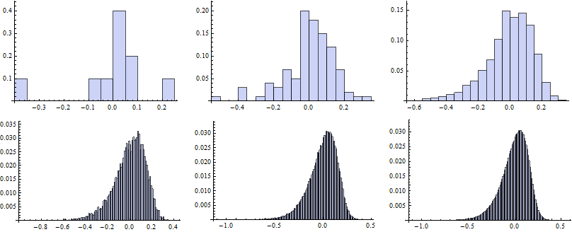
To draw the QQ plot we first specify self-defined function to evaluate the CDF for each random number from the data set, specifing the DataRange on the x-axes. Next, we sort the original series of data and map the QQplot function to them.
![]()
![]()
![]()
![]()
![]()
![]()
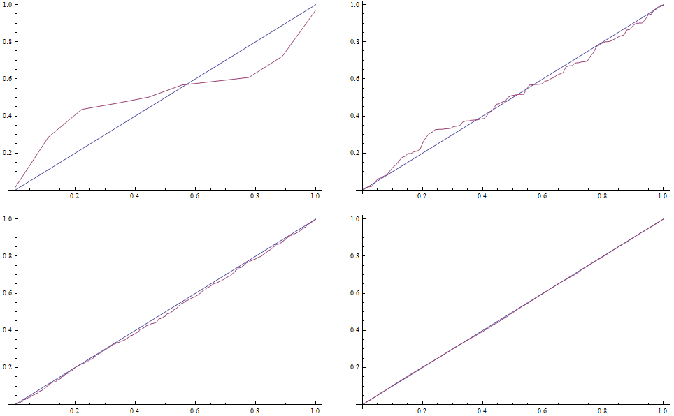
In order to complete the comparison, we can evaluate the Kolmogorov-Smirnov test, ie we look for the widest distance between the simulated distribution function and the teoretical one.
![]()
![]()
AVMC (Monte Carlo with antithetic variates)
The most intuitive utilization of antithetic variates approach to MC simulation is to create a pair of normally distributed variates, keeping the rest of the original PMC algorithm intact.

![]()
![]()
![]()
| Scenarios | Mean | StandardDeviation | Variance | Skewness | Kurtosis | Time |
| 10 | -0.0416492 | 0.175181 | 0.0306883 | -0.885868 | 3.85279 | 0.016 |
| 100 | 0.0025748 | 0.142118 | 0.0201976 | -0.796581 | 4.20435 | 0. |
| 1000 | -0.00108812 | 0.146042 | 0.0213284 | -0.803396 | 3.79889 | 0. |
| 10000 | 0.00054537 | 0.141468 | 0.0200132 | -0.809136 | 4.23777 | 0. |
| 100000 | -0.0000246755 | 0.144275 | 0.0208153 | -0.806563 | 4.15606 | 0.078 |
| 1000000 | 0.0000484112 | 0.144481 | 0.0208749 | -0.802266 | 4.13804 | 0.718 |
| Analytically | 0. | 0.144553 | 0.0208957 | -0.80556 | 4.14235 |
Now we map the Histogram function to vectors of random numbers generated for particular k.
![]()
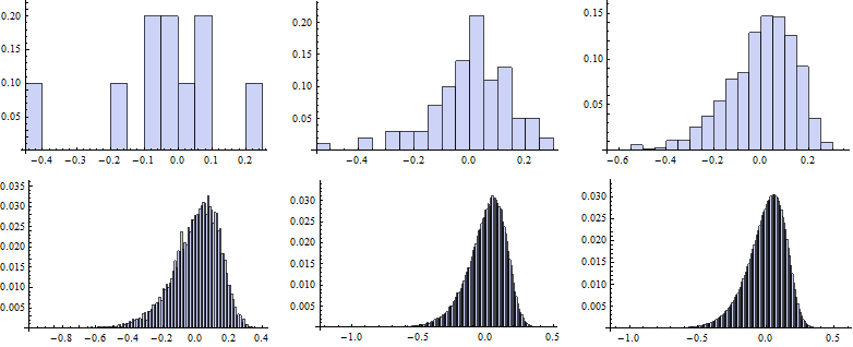
To draw the QQ plot we first specify self-defined function to evaluate the CDF for each random number from the data set, specifing the DataRange on the x-axes. Next, we sort the original series of data and map the QQplot function to them.
![]()
![]()
![]()
![]()
![]()
![]()
In order to complete the comparison, we can evaluate the Kolmogorov-Smirnov test, ie we look for the widest distance between the simulated distribution function and the teoretical one.
![]()
LHSMC (Latin Hypercube Monte Carlo)
The most intuitive utilization of antithetic variates approach to MC simulation is to create a pair of normally distributed variates, keeping the rest of the original PMC algorithm intact.

![]()
![]()
![]()
| Scenarios | Mean | StandardDeviation | Variance | Skewness | Kurtosis | Time |
| 10 | 0.00355704 | 0.1341 | 0.0179828 | -0.00604478 | 1.51669 | 0.016 |
| 100 | -0.00103866 | 0.145109 | 0.0210565 | -0.992879 | 4.77368 | 0.218 |
| 1000 | -0.0000838418 | 0.144901 | 0.0209962 | -0.769672 | 3.79216 | 2.075 |
| 10000 | 0.000282842 | 0.143544 | 0.020605 | -0.818834 | 4.2742 | 20.295 |
| 100000 | -2.21942*10^^-6 | 0.144899 | 0.0209958 | -0.830363 | 4.2689 | 204.799 |
| 1000000 | -0.0000192361 | 0.144652 | 0.0209241 | -0.80708 | 4.14154 | 2052.61 |
| Analytically | 0. | 0.144553 | 0.0208957 | -0.80556 | 4.14235 |
Now we map the Histogram function to vectors of random numbers generated for particular k.
![]()
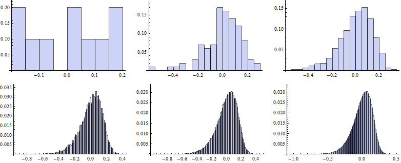
To draw the QQ plot we first specify self-defined function to evaluate the CDF for each random number from the data set, specifing the DataRange on the x-axes. Next, we sort the original series of data and map the QQplot function to them.
![]()
![]()
![]()
![]()
![]()
![]()
In order to complete the comparison, we can evaluate the Kolmogorov-Smirnov test, ie we look for the widest distance between the simulated distribution function and the teoretical one.
![]()
AV-LHSMC (Latin Hypercube Sampled Monte Carlo with antithetic variates)
The most intuitive utilization of antithetic variates approach to MC simulation is to create a pair of normally distributed variates, keeping the rest of the original PMC algorithm intact.

![]()

![]()
![]()
![]()
| Scenarios | Mean | StandardDeviation | Variance | Skewness | Kurtosis | Time |
| 10 | 0.00999564 | 0.108902 | 0.0118597 | 0.456717 | 2.58034 | 0.016 |
| 100 | -0.00815104 | 0.174699 | 0.0305197 | -1.41255 | 6.39834 | 0.281 |
| 1000 | 0.000110044 | 0.144065 | 0.0207548 | -0.788809 | 4.02744 | 2.137 |
| 10000 | 0.0000790131 | 0.143488 | 0.0205887 | -0.768128 | 4.0388 | 21.294 |
| 100000 | -1.2555*10^^-6 | 0.14481 | 0.0209699 | -0.811448 | 4.18621 | 211.74 |
| 1000000 | -0.0000208493 | 0.1446 | 0.0209091 | -0.806458 | 4.14924 | 2196.43 |
| Analytically | 0. | 0.144553 | 0.0208957 | -0.80556 | 4.14235 |
![]()
| Scenarios | Mean | StandardDeviation | Variance | Skewness | Kurtosis | Time |
| 10 | 0.00348365 | 0.109608 | 0.012014 | 0.394537 | 2.12934 | 0.015 |
| 100 | 0.00014285 | 0.146903 | 0.0215806 | -1.29747 | 7.05952 | 0.203 |
| 1000 | 0.000030729 | 0.143368 | 0.0205542 | -0.771469 | 4.11234 | 2.122 |
| 10000 | 3.15478*10^^-6 | 0.144282 | 0.0208173 | -0.804605 | 4.16212 | 21.622 |
| 100000 | 2.66927*10^^-7 | 0.144603 | 0.02091 | -0.800487 | 4.12062 | 210.226 |
| 1000000 | 1.41594*10^^-8 | 0.144509 | 0.0208828 | -0.804002 | 4.13649 | 1967.5 |
| Analytically | 0. | 0.144553 | 0.0208957 | -0.80556 | 4.14235 |
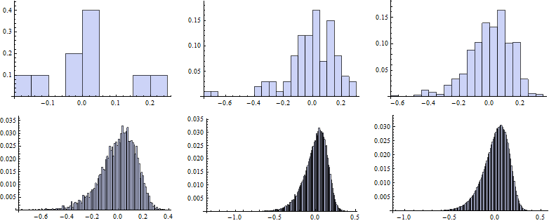
Now we map the Histogram function to vectors of random numbers generated for particular k.
![]()
![]()
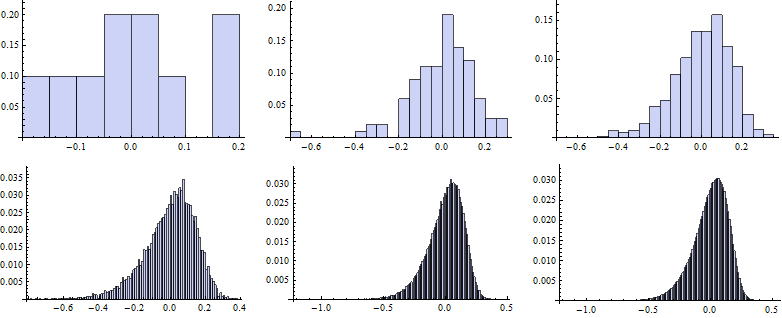
To draw the QQ plot we first specify self-defined function to evaluate the CDF for each random number from the data set, specifing the DataRange on the x-axes. Next, we sort the original series of data and map the QQplot function to them.
![]()
![]()
![]()
![]()
![]()
![]()
In order to complete the comparison, we can evaluate the Kolmogorov-Smirnov test, ie we look for the widest distance between the simulated distribution function and the teoretical one.
![]()
SSMC (Stratified Monte Carlo on the basis of VG distribution function)
The most intuitive utilization of antithetic variates approach to MC simulation is to create a pair of normally distributed variates, keeping the rest of the original PMC algorithm intact.

![]()
![]()
![]()
| Scenarios | Mean | StandardDeviation | Variance | Skewness | Kurtosis | Time |
| 10 | 0.00348365 | 0.109608 | 0.012014 | 0.394537 | 2.12934 | 0.015 |
| 100 | 0.00014285 | 0.146903 | 0.0215806 | -1.29747 | 7.05952 | 0.203 |
| 1000 | 0.000030729 | 0.143368 | 0.0205542 | -0.771469 | 4.11234 | 2.122 |
| 10000 | 3.15478*10^^-6 | 0.144282 | 0.0208173 | -0.804605 | 4.16212 | 21.622 |
| 100000 | 2.66927*10^^-7 | 0.144603 | 0.02091 | -0.800487 | 4.12062 | 210.226 |
| 1000000 | 1.41594*10^^-8 | 0.144509 | 0.0208828 | -0.804002 | 4.13649 | 1967.5 |
| Analytically | 0. | 0.144553 | 0.0208957 | -0.80556 | 4.14235 |
Now we map the Histogram function to vectors of random numbers generated for particular k.
![]()
![]()
To draw the QQ plot we first specify self-defined function to evaluate the CDF for each random number from the data set, specifing the DataRange on the x-axes. Next, we sort the original series of data and map the QQplot function to them.
![]()
![]()
In order to complete the comparison, we can evaluate the Kolmogorov-Smirnov test, ie we look for the widest distance between the simulated distribution function and the teoretical one.
![]()
Inverse Gaussian Distribution
Generally, we proceed in the same way as for the Gamma distribution, though, prespecified algorithm InverseGaussianDistribution can be used.
Normal Inverse Gaussian Distribution
Any of the algorithms that were stated above for Variance Gamma distribution can be used if Gamma distribution is replaced by Inverse Gaussian Distribution.
Plain vanilla call
Note: In this section we provide a sample for estimation of option price by MC approach under BS model. Particular models and approach differes only when error is required to be estimated, too. Otherwise, it is sufficient to replace suitable modul (see above).
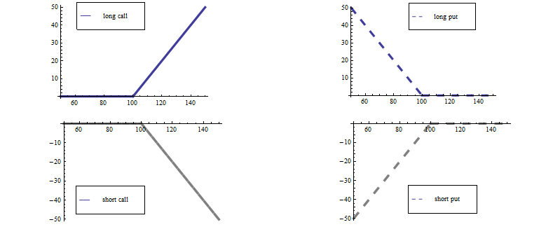
Payoff function
In[25]:=
![]()
In[33]:=

In[34]:=
![]()
Out[34]=
BS model
Inputs (Vstupy)
Here we define basic input data: spot price of the underlying asset, exercise price, time to maturity, riskless rate, dividend rate (costs of cary), volatility of undelying returns, length of one time interval:
In[37]:=
![]()
Within the Black and Scholes model (BS model) the underlying asset price follows the Geometric Brownian motion: ![]() .
.
This gives us:
![]()
![]()
Analytical pricing (Analytické ocenění)
The first formula is the Black and Scholes call option pricing formula, which works also for the maturity time (it includes the payoff function). The second and the third formulas calculate the arguments to the distribution function of the normal distribution, which is defined in the last formula.
In[35]:=

For a given set of input data, the option price is as follows.
In[38]:=
![]()
Out[38]=
![]()
MC - general module
The simplest way to estimate the option price is to apply any of the modules defined above and obtain a vector of N random numbers. After that, terminal price of the underlying asset is calculated and the payoff function is evaluated. It can be done as follows.
In[49]:=

Such a definition of the module allows us to estimate the option price (the mean) and the error of the estimation. The next line gives us the resutls for N = ![]() scenarios, including its error and total time costs, for i=2,3,4,5,6.
scenarios, including its error and total time costs, for i=2,3,4,5,6.
In[51]:=
![]()
Out[51]//MatrixForm=
